Pre-lab (PDF)
Lab 9 Description (PDF)
In this lab, students examine the effects of feedback control on the second order plant of labs 3 and 4 (figure 1 and 2). The controller consists of an op-amp circuit that adds both proportional and derivative control. Proportional control enables the stiffness to be increased (faster rise time), but the damping ratio to be decreased. The larger overshoot and settling time caused by this lower damping ratio is reduced by derivative control. Derivative control (along with proportional control) enables the damping ratio to be increased.
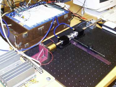
Figure 1. The second-order system, amplifier (bottom left) and breadboard (top).
We fix R2 = 470 kω, Ra = 1 kω and C = 0.1 μF. R1 is set to produce a specified gain. Here we choose R1+R2 >> Ra so that the loading on the RaC network can be ignored. We use the very common LM 741 op-amp in these circuits. Most op-amps are well-modeled an integrator with a high gain (transfer function: a(s) = G/s). For the 741, G is approximately 6 x 10⁶. The circuits in figure 1 can be modeled by the following block diagrams in figure 2.
Figure 2. Drawing of the second-order system used in this lab
In figure 3, the op-amp circuit of this lab is shown. This circuit allows us to implement proportional and lead control with an adjustable gain. The left op-amp is used to create the summation point.
Figure 3. Op-amp circuit for implementation of proportional and lead control with an adjustable gain
The inputs of the first op-amp are switched compared to its equivalent block diagram in figure 4 to compensate for the second inverting op-amp. Students can compare this PD-control with proportional control by leaving the capacitor and R3 out.
Figure 4. Block diagram equivalent of Figure 3
Figure 5 shows the bode plot of this controller. The values of the resistors and capacitor are:
R1 = 68 kω
R2 = 68 kω (1 Mω potentiometer in figure 5 used to create unity gain at low frequencies)
R3 = 6.8 kω
C = 0.47 μF
Figure 5 shows the approximations for lower and higher frequencies. Below the break frequency 1/C(R1+R3) the system's transfer function approaches R2/R1. Above the second break frequency 1/R3 the system's transfer function approaches R2/R1//R3 = R2(R1+R3)/R1R3.
Students can adjust the potentiometer to obtain different rise times with both the P-controller and the PD-controller. They can estimate the position of the poles at each setting, thus creating root-locus plots. Finally, the students can compare the plot of the proportional controlled system with the PD-controlled system.
Figure 5. Bode plot of the controller used in this lab, with approximations for lower and higher frequencies