Lab 8 Description (PDF)
The second-order system that was used in labs 3 and 4 is reused in this lab. By coupling an additional spring and mass to this second-order system, a fourth-order system is constructed as shown in figure 1 and 2. As in lab 3, the bearing shaft with attached collars, LVDT core and voice coil forms a lumped mass m1. The slender spring rod can be modeled as a massless spring k1. The voice coil serves as a force actuator as well as a damper c1. The additional mass m2 is attached to this system via a thin aluminum blade that can be reasonably modeled as a massless spring k2 with light damping c2. This model is shown in figure 3.The voice coil exerts a force Fi on the bearing shaft m1. The LVDT produces a voltage v1 that is proportional to its displacement x1.

Figure 1. Fourth order system consisting of Lab 3 second order system with additional spring and mass
We fix R2 = 470 kω, Ra = 1 kω and C = 0.1 μF. R1 is set to produce a specified gain. Here we choose R1+R2 >> Ra so that the loading on the RaC network can be ignored. We use the very common LM 741 op-amp in these circuits. Most op-amps are well-modeled an integrator with a high gain (transfer function: a(s) = G/s). For the 741, G is approximately 6 x 10⁶. The circuits in figure 1 can be modeled by the following block diagrams in figure 2.
Figure 2. Drawing of the system used in this lab
By studying step responses and determining time constants, students can compare their predictions of the circuit behavior with the actual behavior. Circuit (a) is essentially first order. By adding the RC filter inside the loop circuit (b) we realize an underdamped second-order input-output response. After adding this filter, predictions on locations of the poles of circuit (b) can be compared with measurements. The actual frequency response can be measured easily by using the function generator to provide a sine input. As described in lab 6, differences in magnitude and phase between input and output can be made clear by an oscilloscope that shows both the sine wave input and output. This is most readily accomplished if the oscilloscope can automatically measure magnitude and phase, as shown on the screen.
Figure 3. The sine input and output, showing the magnitude and fase shift at a certain frequency
After disconnecting the dSPACE interface, a function generator can be used to drive the system at an adjustable frequency. The most interesting frequencies are the two resonant frequencies corresponding to complex pole pairs and the frequency of the complex zeros. At the frequency corresponding to the first complex pole pair, both masses will move without much phase difference. This is still visible with the naked eye without using a stroscope. At the frequency of the complex zeros, there will be a phase lag of 90 degrees of the second mass relative to the first mass. However, at this frequency the second mass acts as a vibration absorber so that the first mass hardly moves. At the frequency of the second complex pole pair, the second mass moves in the opposite direction of the first mass. At this frequency, the mode shape of the system can be visualized using a stroboscope, as shown in figure 4.
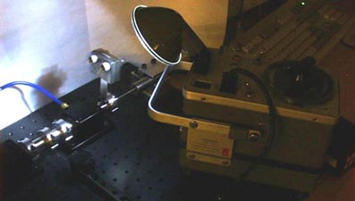
Figure 4. A stroboscope can be used to visualize the mode shapes of the system.
Students use a PC-based measurement system that uses a dSPACE interface to obtain the frequency response graph. This measurement system generates sine wave inputs of different frequencies and measures the output of the system via the LVDT sensor. We use a program written in MATLAB that calculates the amplitude and phase of the system transfer function. An example of these measurements is shown in figures 5 and 6 as red dots.
Figure 5. The theoretical transfer function is shown above, relating the voltage V1 produced by the LVDT to the voltage V produced by the function generator. Its bode plot is shown below (blue lines) along with experimental values (red dots).
The values of the constants in this equation are:
K = 1400
ωn1 = 31 rad/s (4.93 Hz), ζ1 = 0.17
ωn2 = 67.4 rad/s (10.7 Hz), ζ2 = 0.042
ωz = 56.01 rad/s (8.91 Hz), ζz = 0.001
Obviously, there is a significant difference between the actual system and the theoretical one. This is caused by a nonlinear
dynamic in the voice coil. If a pole is added at 150 rad/s (24 Hz) to compensate for these nonlinearities, the difference
becomes much smaller, as shown in figure 6.

Figure 6. The transfer function of figure 5 with an added pole at 150 rad/s (24 Hz) (blue line) and the measured values (red dots).